Gauss Elimination#
강좌: 수치해석
Numpy array#
Python 에서 Array, Matrix는 Numpy 패키지로 사용할 수 있다.
몇가지 특징을 살펴보면 다음과 같다.
생성
import numpy as np

A = np.array([[1, 2, 3], [4, 5, 6]])

# Array 출력
print(A)

# Array 차원, 크기
print(A.ndim, A.shape)
[[1 2 3]
 [4 5 6]]
2 (2, 3)
Indexing
Zero-based Numbering: Index는 0 부터 시작
# 2행, 1열의 값 a_{21}
print(A[1, 0])
4
# 2번째 행
print(A[1])
[4 5 6]
# 3번째 열
print(A[:, 2])
[3 6]
연산
합, 차
Scalar 곱
B = np.array([[1, 1, 1], [2, 2, 2]])

# Array B 출력
print(B)
[[1 1 1]
 [2 2 2]]
# 합
A + B
array([[2, 3, 4],
       [6, 7, 8]])
# 차
A - B
array([[0, 1, 2],
       [2, 3, 4]])
# Scalar 곱
c = 5
c*A
array([[ 5, 10, 15],
       [20, 25, 30]])
내적 (Inner product)
np.dot또는@연산
x = np.array([2,1,3])

# Inner product
A @ x
array([13, 31])
# Elementwise production
A*x
array([[ 2,  2,  9],
       [ 8,  5, 18]])
Transpose
A.T
array([[1, 4],
       [2, 5],
       [3, 6]])
Gauss 소거법#
연립방정식 소거법을 적용
Forward elimination: Upper triangular matrix 구성
\[ a_{j,k} - \frac{a_{j, i}}{a_{i,i}} \times a_{i,k} ~~~ \textrm{for}~~j > i~~\textrm{and}~~k\geq i \]Backward substitution
\[ x_i = \frac{1}{a_{i,i}} \left (\tilde{b}_i - \sum_{j=i+1}^n a_{i,j} x_j \right ) \]
By hand#
예제
# Make matrix, array
A = np.array([[2, 1, 1], [4, -6, 0], [-2, 7, 2]])
b = np.array([5, -2, 9])

print(A, b.T)
[[ 2  1  1]
 [ 4 -6  0]
 [-2  7  2]] [ 5 -2  9]
# first pivot a_{1,1}
# eliminate a_{2,1}
i = 0
j = 1
ratio = A[j, i] / A[i, i]

A[j] = A[j] - ratio*A[i]
b[j] = b[j] - ratio*b[i]

print(A[j], b[j])
[ 0 -8 -2] -12
# eliminate a_{3,1}
j = 2
ratio = A[j, i] / A[i, i]

A[j] = A[j] - ratio*A[i]
b[j] = b[j] - ratio*b[i]

print(A[j], b[j])
[0 8 3] 14
# next pivot a_{2,2}
# eliminate a_{3, 2}
i = 1
j = 2

ratio = A[j, i] / A[i, i]

A[j, i:] = A[j, i:] - ratio*A[i, i:]
b[j] = b[j] - ratio*b[i]

print(A[j], b[j])
[0 0 1] 2
print(A, b[:, None])
[[ 2  1  1]
 [ 0 -8 -2]
 [ 0  0  1]] [[  5]
 [-12]
 [  2]]
Forward elimination 결과
x = np.empty_like(b)

# Third row
i = 2
xi = b[i] / A[i,i]
x[i] = xi
print(x[i])
2
# Second row
i = 1
xi = (b[i] - A[i, i+1]*x[i+1]) / A[i, i]
x[i] = xi
print(x[i])
1
# First row
n = 3
i = 0
xi = b[i]

for j in range(i+1, n):
    xi -= A[i, j]*x[j]

xi /= A[i,i]

x[i] = xi
print(x[i])
1
# Solution
print(x)

# 검산
A = np.array([[2, 1, 1], [4, -6, 0], [-2, 7, 2]])
print(A @ x)
[1 1 2]
[ 5 -2  9]
Python code#
def gauss_eliminate(A, b):
    """
    Gauss Elimination

    Parameters
    ----------
    a : matrix
        Linear operator
    b : array
        Result

    Returns
    --------
    x : array
        Solution
    """

    # Check size
    m, n = np.array(A).shape
    l = len(b)

    if (m != n) or (n != l) or (m != l):
        raise ValueError('Wrong shape', m,n,l)

    # Forward elimiation
    for i in range(n):
        if A[i, i] == 0.0:
            raise ValueError('Pivot is zero')

        for j in range(i+1, n):
            ratio = A[j, i] / A[i, i]

            #A[j, i:] = A[j, i:] - ratio*A[i, i:]
            for k in range(i+1, n):
                A[j, k] = A[j, k] - ratio*A[i, k]
            b[j] = b[j] - ratio*b[i]

    # Back substitution
    x = np.empty(n)

    for i in range(n-1, -1, -1):
        x[i] = b[i]

        for j in range(i+1, n):
            x[i] -= A[i, j]*x[j]

        x[i] /= A[i,i]

    return x
A = np.array([[2, 1, 1], [4, -6, 0], [-2, 7, 2]])
b = np.array([5, -2, 9])

x = gauss_eliminate(A, b)
print(x)
[1. 1. 2.]
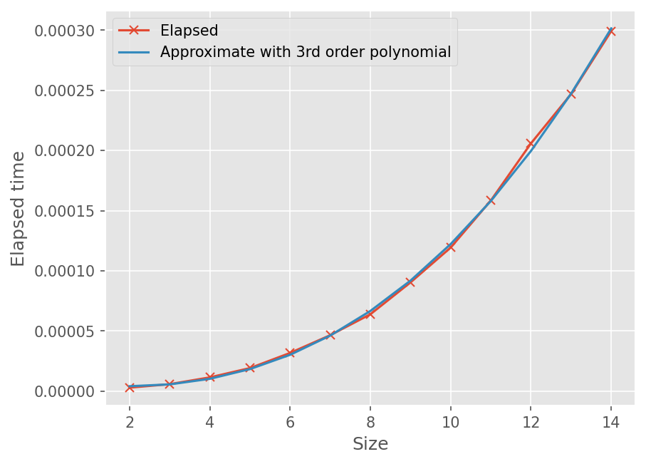
Computational Costs#
Gauss Elimination 코드 계산 시간 확인
size = np.arange(2, 15)
elapsed = []

for n in size:
    a = np.random.rand(n, n)
    b = np.random.rand(n)

    print("Size of matrix : ", n)
    t = %timeit -o gauss_eliminate(a, b)
    elapsed.append(t.average)
Size of matrix :  2
2.93 μs ± 198 ns per loop (mean ± std. dev. of 7 runs, 100,000 loops each)
Size of matrix :  3
5.82 μs ± 163 ns per loop (mean ± std. dev. of 7 runs, 100,000 loops each)
Size of matrix :  4
11.5 μs ± 238 ns per loop (mean ± std. dev. of 7 runs, 100,000 loops each)
Size of matrix :  5
19.2 μs ± 613 ns per loop (mean ± std. dev. of 7 runs, 100,000 loops each)
Size of matrix :  6
31.8 μs ± 1.82 μs per loop (mean ± std. dev. of 7 runs, 10,000 loops each)
Size of matrix :  7
46.5 μs ± 4.63 μs per loop (mean ± std. dev. of 7 runs, 10,000 loops each)
Size of matrix :  8
63.9 μs ± 2.84 μs per loop (mean ± std. dev. of 7 runs, 10,000 loops each)
Size of matrix :  9
90.4 μs ± 3.98 μs per loop (mean ± std. dev. of 7 runs, 10,000 loops each)
Size of matrix :  10
119 μs ± 1.8 μs per loop (mean ± std. dev. of 7 runs, 10,000 loops each)
Size of matrix :  11
158 μs ± 3.06 μs per loop (mean ± std. dev. of 7 runs, 10,000 loops each)
Size of matrix :  12
206 μs ± 8.85 μs per loop (mean ± std. dev. of 7 runs, 1,000 loops each)
Size of matrix :  13
247 μs ± 15.6 μs per loop (mean ± std. dev. of 7 runs, 1,000 loops each)
Size of matrix :  14
299 μs ± 12.7 μs per loop (mean ± std. dev. of 7 runs, 1,000 loops each)
%matplotlib inline
from matplotlib import pyplot as plt

import numpy as np

plt.style.use('ggplot')
plt.rcParams['figure.dpi'] = 150
fig, ax = plt.subplots()
ax.plot(size, elapsed, marker='x')

# Approximate elapsed time with 3rd order polynomial
z = np.polyfit(size, elapsed, 3)
appxf = np.poly1d(z)

ax.plot(size, appxf(size))
ax.legend(['Elapsed', 'Approximate with 3rd order polynomial'])
ax.set_xlabel('Size')
ax.set_ylabel('Elapsed time')
Text(0, 0.5, 'Elapsed time')
Forward elimination
첫번째 pivot (이후 n-1 rows)
each row: n번 Add/sub, n+1번 Mul
두번째 pivot (이후 n-2 rows)
each row: (n-1)번 Add/sub, n번 Mul
…
마지막 pivot (마지막 row)
last row: 2번 Add/sub, 3번 Mul
Total
Add/Sub
\[ \sum_{k=1}^{n-1} (n-k)(n+1-k)= \frac{1}{3} n^3 - \frac{1}{3} n \]Mul
\[ \sum_{k=1}^{n-1} (n-k)(n+2-k)= \frac{1}{3} n^3 + \frac{5}{2} n^2 - \frac{17}{6} \]All : \(\frac{2}{3} n^3 + O(n^2)\)
Backward substitution
\(O(n^2)\)
문제점#
Round-off Error
Pivot이 0일 때
Row exchange 필요
ill-conditioned system
2x2 선형 방정식
\[\begin{split} \left [ \begin{matrix} 1 & 1 \\ 1 & 1+\epsilon_1 \end{matrix} \right ] \left [ \begin{matrix} x \\ y \end{matrix} \right ] = \left [ \begin{matrix} 2 \\ 2 + \epsilon_2 \end{matrix} \right ] \end{split}\]\(\epsilon_2=0\) : \((x,y) = (2, 0)\)
\(\epsilon_2 \ne 0\) : \((x,y) = (1, 1)\)
e1 = 1e-3
a = np.array([[1, 1], [1, 1+e1]])
b = np.array([2, 2])

gauss_eliminate(a, b)
array([2., 0.])
e1 = 1e-3
a = np.array([[1, 1], [1, 1+e1]])
b = np.array([2, 2+e1])

gauss_eliminate(a, b)
array([1., 1.])
for n in range(1, 16):
    e1 = 10**(-n)

    a = np.array([[1, 1], [1, 1+e1]])
    b = np.array([2, 2+e1])

    x = gauss_eliminate(a, b)
    print("Exponent of e2: -{}, Sol : {}".format(n, x))
Exponent of e2: -1, Sol : [1. 1.]
Exponent of e2: -2, Sol : [1. 1.]
Exponent of e2: -3, Sol : [1. 1.]
Exponent of e2: -4, Sol : [1. 1.]
Exponent of e2: -5, Sol : [1. 1.]
Exponent of e2: -6, Sol : [1. 1.]
Exponent of e2: -7, Sol : [1. 1.]
Exponent of e2: -8, Sol : [1. 1.]
Exponent of e2: -9, Sol : [1. 1.]
Exponent of e2: -10, Sol : [1. 1.]
Exponent of e2: -11, Sol : [1. 1.]
Exponent of e2: -12, Sol : [1. 1.]
Exponent of e2: -13, Sol : [1. 1.]
Exponent of e2: -14, Sol : [0.97777778 1.02222222]
Exponent of e2: -15, Sol : [1.2 0.8]
Pivoting#
계산의 순서를 바꾸서 Round-off 오차에 의한 연산 오류를 최소화 함.
종류
Partial pivoting: \(i\) 번째 컬럼 (부분 행렬에서 첫번째) 에서 절대값이 가장 큰 row를 Pivot row로 설정
Complete pivoting: 부분 행렬에서 크기가 가장 큰 성분을 포함하는 row를 Pivot row로 설정
미지수도 재배치 됨
Scaling
각 row 계수의 크기를 표준화해서 오차를 줄임
Scaled partial pivoting
각 row에서 계수의 크기가 최대인 값을 factor로 지정: \(s_i = \max_{j}|a_{ij}|\)
j 번째 Pivot을 정할 때 \(|a_{ij}|/s_i\) 가 최대인 row를 선택해서 Pivot row로 설정
예제#
다음 선형 방정식을 계산하시오.
# Gauss elimination
A = np.array([[0.0003, 3.0], [1, 1]], dtype=np.float32)
b = np.array([2.0001, 1.0], dtype=np.float32)

gauss_eliminate(A, b)
array([0.3334796 , 0.66666662])
# Swap first and second row (Partial pivoting)
A = np.array([[1, 1], [0.0003, 3.0]], dtype=np.float32)
b = np.array([1.0, 2.0001], dtype=np.float32)

gauss_eliminate(A, b)
array([0.3333334, 0.6666666])
# Scaled
A = np.array([[3.0, 30000.0], [1, 1]], dtype=np.float32)
b = np.array([20001, 1.0], dtype=np.float32)

gauss_eliminate(A, b)
array([0.33333333, 0.66666667])
예제#
다음 선형방정식을 Paritial Pivot 기법을 이용하여 계산하시오.
by hand#
A = np.array([
    [3, -13, 9, 3],
    [-6, 4, 1, -18],
    [6, -2, 2, 4],
    [12, -8, 6, 10]
], dtype=float)

b = np.array([-19, -34, 16, 26], dtype=float)
n = 4
# 첫번째 Pivot 결정
i = 0
print(abs(A[:, i]))

# 4번째 row를 Pivot로 결정
j = np.argmax(abs(A[:, i]))

# Swap rows (A and b)
for k in range(i, n):
    tmp = A[i, k]
    A[i, k] = A[j, k]
    A[j, k] = tmp

tmp = b[i]
b[i] = b[j]
b[j] = tmp
[ 3. 6. 6. 12.]
A, b
(array([[ 12.,  -8.,   6.,  10.],
        [ -6.,   4.,   1., -18.],
        [  6.,  -2.,   2.,   4.],
        [  3., -13.,   9.,   3.]]),
 array([ 26., -34.,  16., -19.]))
# Row operations
for j in range(i+1, n):
    ratio = A[j, i] / A[i, i]

    A[j, i:] = A[j, i:] - ratio*A[i, i:]
    b[j] = b[j] - ratio*b[i]
A, b
(array([[ 12. ,  -8. ,   6. ,  10. ],
        [  0. ,   0. ,   4. , -13. ],
        [  0. ,   2. ,  -1. ,  -1. ],
        [  0. , -11. ,   7.5,   0.5]]),
 array([ 26. , -21. ,   3. , -25.5]))
# 두번째 Pivot 결정
i = 1
print(abs(A[i:, i]))

# 1, 2, 3 행에서 scaled 값 비교
j = np.argmax(abs(A[i:, i])) + i

# Swap rows (A and b)
for k in range(i, n):
    tmp = A[i, k]
    A[i, k] = A[j, k]
    A[j, k] = tmp

tmp = b[i]
b[i] = b[j]
b[j] = tmp
[ 0. 2. 11.]
A, b
(array([[ 12. ,  -8. ,   6. ,  10. ],
        [  0. , -11. ,   7.5,   0.5],
        [  0. ,   2. ,  -1. ,  -1. ],
        [  0. ,   0. ,   4. , -13. ]]),
 array([ 26. , -25.5,   3. , -21. ]))
# Row operations
for j in range(i+1, n):
    ratio = A[j, i] / A[i, i]

    A[j, i:] = A[j, i:] - ratio*A[i, i:]
    b[j] = b[j] - ratio*b[i]
# 두번째 Pivot 결정
i = 2
print(abs(A[i:, i]))

# 2, 3 행에서 scaled 값 비교
j = np.argmax(abs(A[i:, i])) + i

# Swap rows (A and b)
for k in range(i, n):
    tmp = A[i, k]
    A[i, k] = A[j, k]
    A[j, k] = tmp

tmp = b[i]
b[i] = b[j]
b[j] = tmp
[0.36363636 4. ]
# Row operations
for j in range(i+1, n):
    ratio = A[j, i] / A[i, i]

    A[j, i:] = A[j, i:] - ratio*A[i, i:]
    b[j] = b[j] - ratio*b[i]
A, b
(array([[ 12.        ,  -8.        ,   6.        ,  10.        ],
        [  0.        , -11.        ,   7.5       ,   0.5       ],
        [  0.        ,   0.        ,   4.        , -13.        ],
        [  0.        ,   0.        ,   0.        ,   0.27272727]]),
 array([ 26.        , -25.5       , -21.        ,   0.27272727]))
# Back substitution
x = np.empty_like(b)

for i in range(n-1, -1, -1):
    x[i] = b[i]

    for j in range(i+1, n):
        x[i] -= A[i, j]*x[j]

    x[i] /= A[i,i]
x
array([ 3., 1., -2., 1.])
# Validation
A = np.array([
    [3, -13, 9, 3],
    [-6, 4, 1, -18],
    [6, -2, 2, 4],
    [12, -8, 6, 10]
])

A @ x
array([-19., -34., 16., 26.])
DIY#
Partial Pivot을 하는 Gauss Elimination 함수를 작성하시요.